This year, we’ve been participating in the CollegeFootballData.com prediction contest, where each week you predict the actual spread of the game. You’re judged on a variety of factors like your outright picks, picks against the spread, absolute and mean-squared error. Two areas that we are performing very well (1st and 2nd, respectively), are MSE and absolute error. Today, I’ll show you how we do that.
Getting the Data
We’ll be using R today, and we’ll be getting all of our data from the collegefootballdata.com API. This part requires you to have your own API key from CFB Data. If you don’t have one yet, you can get one here. This also requires you to store your key. I recommend storing it in your .Renviron file, which you can probably find in your Documents folder on Windows.

Then, you’ll want to edit it in Notepad and add your key like this:
cfbd_staturdays_key = "yoursecretkey"
Now, you should be all set to do the rest of the exercise. Let’s first grab a few functions that will help us get the data from the API.
# Load in required functions
source(https://raw.githubusercontent.com/kylebennison/staturdays/master/Production/source_everything.R)
Next, let’s get the initial data. We’ll need the games, elo ratings, and betting data.
# Get historic Elo data from Staturdays
elo <- get_elo(2013, 2021)

# Get games data from CFBdata
games <- get_games(2013, 2021)

# Get historic betting data from CFBdata
betting.master = data.frame()
for(j in 2013:2021){
  message("Doing year ", j)
betting_url <- paste0("https://api.collegefootballdata.com/lines?year=", j)
full_url_betting <- paste0(betting_url)
full_url_betting_encoded <- URLencode(full_url_betting)
betting <- cfbd_api(full_url_betting_encoded, my_key)
betting <- as_tibble(betting)
betting <- unnest(betting, cols = c(lines))
betting.master = rbind(betting.master, betting)
}
Cleaning the Data
We’ll have to do some clean up to get the data ready to use in a model. First, we’ll average out the data in the betting file, because we have multiple lines from different providers for the same game, so we’ll just take the average of all the lines.
Next, we’ll create a new field called “join_date” in our Elo file, since the Elo is from after the game is finished in that week, so we’ll want to join each Elo rating to the following week’s game.
Then, we’ll join all three tables (games, elo, and betting) together.
# Need to summarise lines for teams with multiple lines
betting_consensus <- betting.master %>%
  mutate(spread = as.double(spread),
         overUnder = as.double(overUnder)) %>%
  group_by(id, season, week, homeTeam, awayTeam,
           homeConference, awayConference, homeScore, awayScore) %>%
  summarise(consensus_spread = mean(spread, na.rm = TRUE),
            consensus_over_under = mean(overUnder, na.rm = TRUE),
            consensus_home_ml = mean(homeMoneyline, na.rm = TRUE),
            consensus_away_ml = mean(awayMoneyline, na.rm = TRUE))

e2 <- elo %>%
  group_by(team) %>%
  mutate(join_date = lead(date, n = 1L, order_by = date))

games_elo <- games %>%
  mutate(start_date = lubridate::as_datetime(start_date)) %>%
  left_join(e2, by = c("start_date" = "join_date",
                       "home_team" = "team")) %>%
  left_join(e2, by = c("start_date" = "join_date",
                       "away_team" = "team"),
            suffix = c("_home", "_away"))

games_elo_lines <- games_elo %>%
  inner_join(betting_consensus, by = "id")
Doing Some Calculations
Ok, we’ve cleaned everything up and joined it together. Now, we need to do some calculations. Mainly, we want to know the difference in Elo between the home and away teams, since we’ll use this as a feature in our model later. We’ll also want to calculate the final actual spread of the game, and this will be our response variable: the variable we’re trying to predict.
ge2 <- games_elo_lines %>%
  mutate(home_elo_adv = elo_rating_home + 55 - elo_rating_away,
         final_home_spread = away_points - home_points)
We’re including a 55 point home-field advantage in the Elo advantage calculation, which we’ve identified as the best home-field advantage value in previous testing.
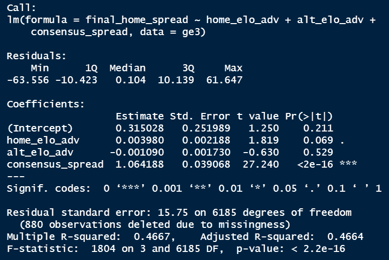
Let’s look at the relationship between Elo and the final spread.
ge2 %>%
  ggplot(aes(x = home_elo_adv, y = final_home_spread)) +
  geom_point(alpha = .1, color = staturdays_colors("light_blue")) +
  geom_smooth(color = staturdays_colors("orange")) +
  staturdays_theme +
  theme(panel.grid.major = element_line(color = "lightgrey")) +
  labs(title = "Elo and Spread 2000-2021",
       subtitle = "Elo advantage includes built-in home-field advantage worth around 3 points",
       x = "Home Elo Point Advantage/Disadvantage",
       y = "Home Win/Loss Point Margin")
So remember that a negative spread means the home team won by that amount. So, as the Elo advantage increases for home teams, so does the spread. There is a lot of deviation, but the relationship is clearly linear. So we should be able to model this, and we’ll use a linear regression model.
Now, CFB Data recently provided their own Elo model, and while it’s fairly similar to Staturdays, it is different in a few decisions and assumptions it makes. Rather than be picky, I’m just going to include them both. It can only help our model if you think of it like the wisdom of the crowd (this isn’t really true if two variables are highly correlated, it can actually throw off your model and make it worse). Of course, this isn’t always true. More variables doesn’t always mean a better model if those variables aren’t helpful. If I include the time of the kickoff as a variable, it might end up confusing the model more than helping it because it might find some strange correlation that has nothing to do with the team’s or their skill and more to do with random chance.
# Include CFB Data's elo as well.
ge3 <- ge2 %>% mutate(alt_elo_adv = home_pregame_elo - away_pregame_elo)
Ok, we’re ready to build our model.
Building the Linear Regression Model
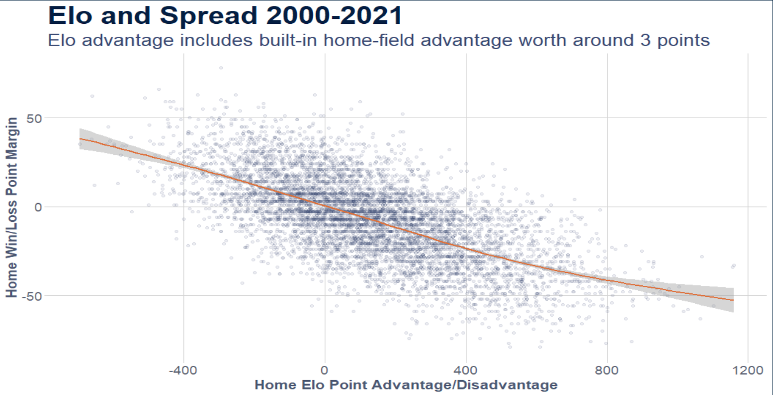
model_spread <- lm(final_home_spread ~ home_elo_adv + alt_elo_adv + consensus_spread, ge3)

summary(model_spread)
So the lm() function is to build a linear model, and the syntax you’re seeing is saying “predict final_home_spread using home_elo_adv, alt_elo_adv, and consensus_spread, from the ge3 dataset”. Here are the results.

So we have an R-squared of .47, which means 47% of the variation in spread can be explained by our model. That’s not great, but it’s certainly a start. The consensus spread is the only variable that is significant at the 5% confidence level, but that doesn’t mean we need to exclude our other variables. We would want to compare the results to a model that excluded elo and see which performed better. For now, we’ll leave it as is.
If you really wanted to stress-test your model’s validity in the real world, you could train and test it, using a holdout set of data. We’ve skipped this because we’re just trying to build a model here, and not necessarily test and optimize it right now.
Saving and Using The Model
Now that we have the model, we can apply it to new data to get predictions.
If you want to save a model for use another time, you can save it to a .rds file.
saveRDS(model_spread, file = "Production Models/elo_combo_spread_model_v2.rds")
To apply this model, we’d need to rerun all the code above, but only pull data from 2021 and look at the games coming up this week. Then, we’d run this code to make our spread predictions:
# Read in the model we saved earlier
model_spread <- readRDS(file = "Production Models/elo_combo_spread_model_v2.rds")

# Predict the spread using our model
ge3$predicted_spread <- predict(model_spread, newdata = ge3)
And there you have it. R will use your model and the input variables in your ge3 data to predict the final spread of the game!
From here, we could try to include more relevant variables that might help improve our model, or we could try a different model type altogether, like a decision tree, to see if that helps predict spreads more accurately.

Leave a comment